Backtesting in Workbench
Discover Workbench's new backtesting suite and take your investment strategy to the next level. Test and compare trading hypotheses, and evaluate risk and performance with metrics like drawdown and Sharpe ratio. Explore basic and advanced trading strategy examples, including on-chain indicators.


This article introduces a backtesting suite for our Workbench tool. Workbench lets users quickly compare existing metrics, apply formulas, and derive new custom metrics. We will demonstrate how trading strategies can be defined within Workbench and how a simulation of such self-defined trading strategies on historical data can be run.
Introduction
In its narrowest definition, a backtest is a historical simulation of how an investment strategy would have performed should it have been run over a past period. A strategy is a set of rules that specify when an asset should be bought and sold. A practical way of representing an investment strategy is in terms of a so-called trading signal. A trading signal is a real-valued function of time, which returns values in the range [0, 1] or, equivalently, 0-100%. The trading signal dictates how much of the trading portfolio should be invested in the underlying asset for each instance of time. For example, the HODL strategy is represented with a constant signal of 1; we hold 100% of our investment capital in bitcoin over time. For advanced traders, a short position of an asset is represented by a negative trading signal: a signal of -1 equals a short position with a size of 100% of the investment portfolio. Including short positions, the valid range for the trading signal extends to [-1, 1].
It should be understood, however, that a backtest will never coincide with the live performance of a trading strategy. The biggest pitfall when backtesting is backtest overfitting. Tuning the parameters of a strategy towards the best historical performance (in-sample) will likely reduce the generality of the strategy and thus decrease future performance (out-of-sample). But many difficulties remain even when accounting for backtest overfitting (as far as possible). Luo et al. offer a summary of common backtesting mistakes in their article “Seven Sins of Quantitative Investing” (Luo et al. [2014]). Backtesting is not a research tool and is unsuited for deriving trading strategies. It merely serves as the last step within a research process to ultimately test and potentially invalidate an investment hypothesis.
See Backtesting in action through the video guide
The Backtesting Suite
Before looking at some concrete examples, we discuss the general outline of defining trading strategies and simulating them over the past. Running a backtest in Workbench always follows the same procedure:
- The trading strategy has to be translated to a trading signal which assigns a value between zero and one to each point in time. Let’s abbreviate the trading signal with
f1. - Call the new Workbench
backtestfunction:
backtest(m1, f1, since, initial_capital_usd, rel_trading_costs)
Let’s break down what each argument stands for:
m1: the price series (e.g., BTC) you want to trade.f1: the trading signal from the first step.since: a timestamp indicating the start date of your trading simulation, e.g.,"2020-01-01"initial_capital_usd: how much money (USD) you allocate to your strategy for trading, e.g.,1000(USD). Over time, no additional capital flows in or out of the simulated trading portfolio. This is in contrast to, e.g., a dollar cost averaging strategy. Instead, the trading simulation will vary the exposure to the traded asset over time, depending on the trading signal.rel_trading_costs: an approximation of the expected relative trading costs, which consist of exchange fees and slippage. A value of, e.g.,0.001refers to trading costs of 0.1% of the volume of each trade.
The backtest function generates a so-called Net Asset Value (NAV) curve. This represents your portfolio’s value over time (in USD). Your portfolio consists of a mixture of USD and BTC at all times. The trading signal determines which fraction of the portfolio is invested in BTC, and the remainder (one minus trading signal) represents the USD component of your portfolio. The NAV, however, always represents the entire value of the portfolio denominated in USD.
For the experts: under the hood, the backtest function multiplies the previous day’s trading signal with the (daily) return of the underlying (m1, e.g., BTC) for each day while taking trading costs on signal changes into account. The resulting return series is then aggregated and adjusted for initial investment and the starting date of the simulation.
Examples
In the remainder of this document, we will walk you through a few toy examples of defining trading strategies and running the corresponding backtests. In particular, we will start with the most fundamental strategy: buy and hold. After that, we look at a standard technical indicator, the simple moving average cross-over. Finally, we will dive into a more interesting example; we will test a trading hypothesis based on the SOPR on-chain metric.
Example 0: HODL
We will start with the most basic and rightfully most popular trading strategy for Bitcoin: hodling. Imagine you had a lump sum of cash you wanted to invest in bitcoin. The most straightforward way is to buy bitcoin and never sell. This will serve as a baseline to compare with other strategies. In the following, we will adopt this basic investment strategy as a first example of creating a backtest in Workbench.
We have prepared a Workbench preset that constitutes the HODL strategy trading signal and backtest for you.
There, we have defined the trading strategy HODL signal in formula f1 as m1/m1, where m1 is the price of BTC. Thus, the trading signal is constant one over time. When defining the signal, you don’t have to worry about the start date of your simulation; this comes in the next step.
Formula f2 which is labeled as HODL backtest [USD] contains the call to the backtest function:
backtest(m1, f1, "2020-01-01", 1000, 0.001)
The parameters above define your backtest simulation to adopt m1 as the underlying trading asset (BTC) and f1 as the trading signal, starting on "2020-01-01" with an initial portfolio value of $1000 and trading costs of 0.1%. This finalizes our first backtest! Below is a chart with the strategy's resulting NAV curve (labeled as HODL backtest [USD]) and the constant trading signal HODL signal. You can read off the total return of your investment by comparing the value of the NAV chart at the latest date to the starting date.
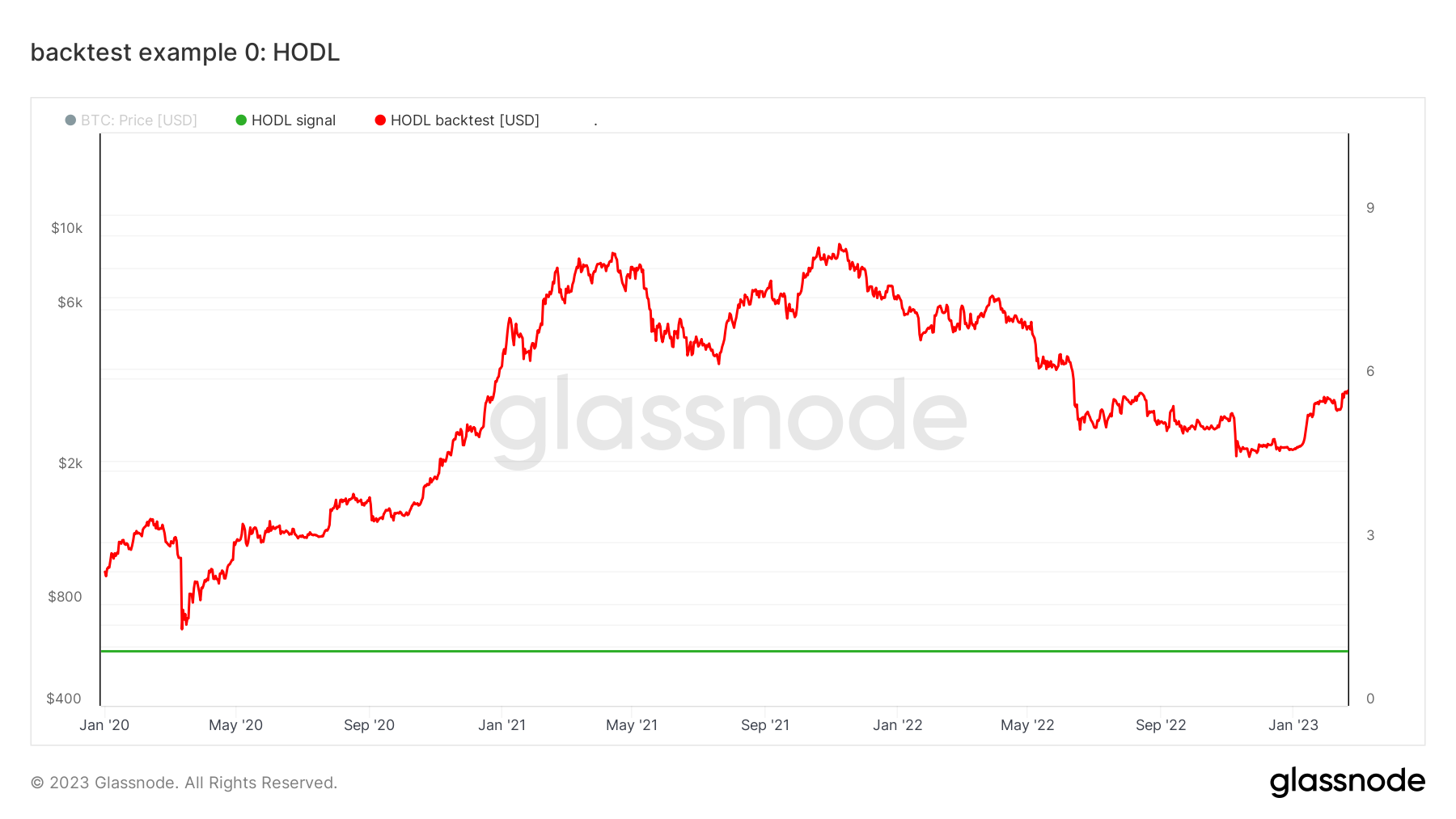
To recap: we have simulated the purchase of $1000 of BTC on January 1st, 2020, with subsequent diamond-hands hodling until the present.
Example 1: Simple Moving Average Cross-Over
You’re here to learn about backtesting. Thus, there is a fair chance that you want to investigate trading strategies beyond hodling. Strategies that constitute a systematic way of buying and selling an asset. Let’s get to it.
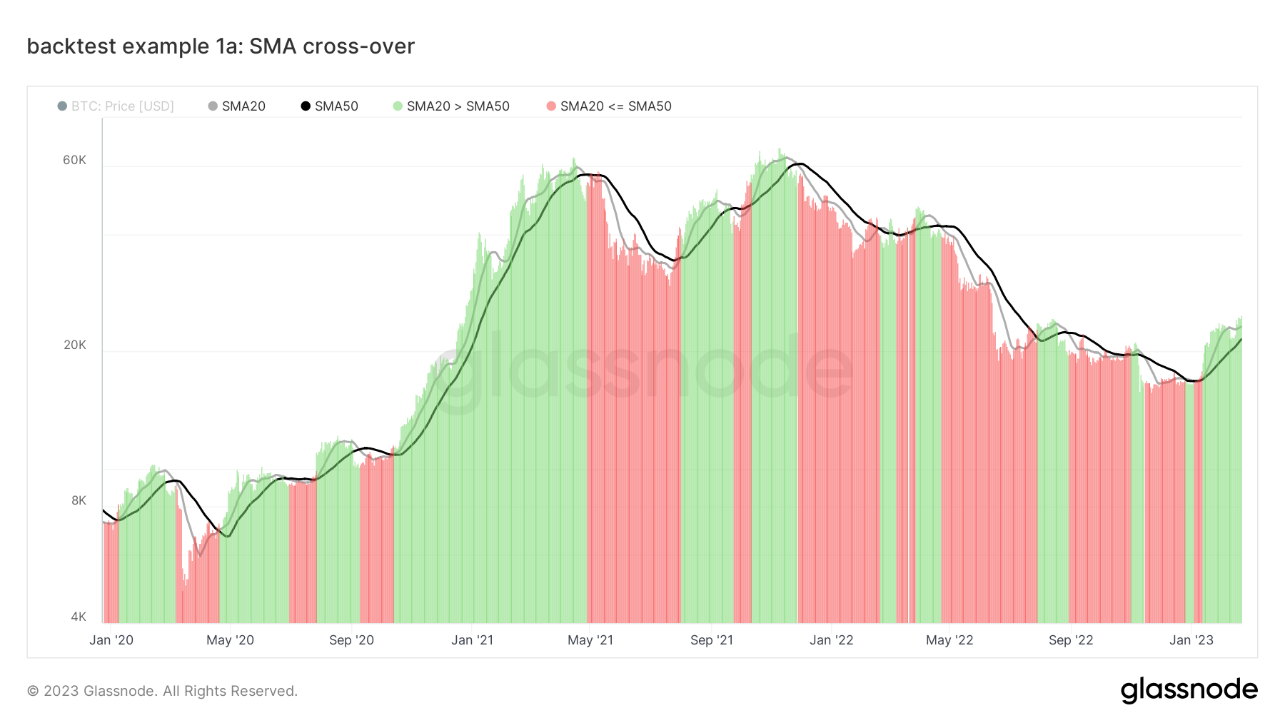
The Simple Moving Average (SMA) cross-over is our first example of a systematic trading strategy. This popular trend-following indicator consists of two SMAs with different periods (e.g., 20 days and 50 days). The motivation is as follows: when the price is in an uptrend, so will the price’s SMAs for all periods. By construction, though, the SMA with a shorter period is quicker to react to an emerging uptrend than the SMA with a longer period. This brings us to our set of trading rules:
- Whenever the shorter SMA is above the longer SMA, we assert that we are in a bullish trend, and we buy and hold bitcoin, i.e., the trading signal is at one or 100%.
- Otherwise (the shorter SMA is below the longer SMA), sell bitcoin and hold cash. The corresponding trading signal is zero.
Purely for the sake of illustration, let’s quickly look at a Python-style pseudo-code to formalize these trading rules:
# SMA cross-over trading rules:
if sma20 > sma50:
    signal = 1
else:
    signal = 0
If you’re more visual, here is a plot of the BTC price (bars) and the two simple moving averages (SMA20 and SMA50). Our set of trading rules determines the color of the price bars. When the trading signal is one, the color is green; when the signal is zero, the color is red.
Now that the trading rules of the SMA cross-over have been laid out, we are prepared to backtest them! This Workbench preset expands on the previous example. We will use the Workbench if conditional (see the Workbench Guide for details). In line with the previously defined trading rules, we define the trading signal f3 as:
if(sma(m1, 20), ">", sma(m1, 50), 1, 0)
Now that we have done the heavy lifting by defining the trading signal, performing a backtest on the SMA cross-over trading strategy is straightforward. This step is identical to creating the backtest of the hodling strategy; we only pass a different signal. Let’s define the backtest (in our example, it is formula f4) via:
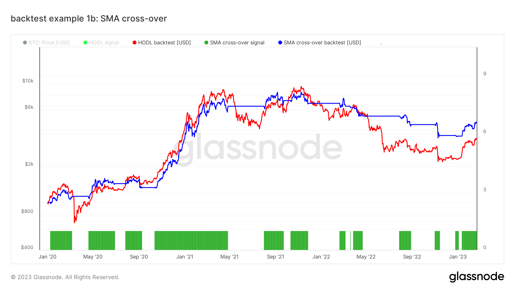
backtest(m1, f3, "2020-01-01", 1000, 0.001)
This directly output the NAV curve of the SMA cross-over trading strategy, labeled in the Workbench preset as SMA cross-over backtest (blue curve). The previously introduced HODL backtest is included in red color for comparison.
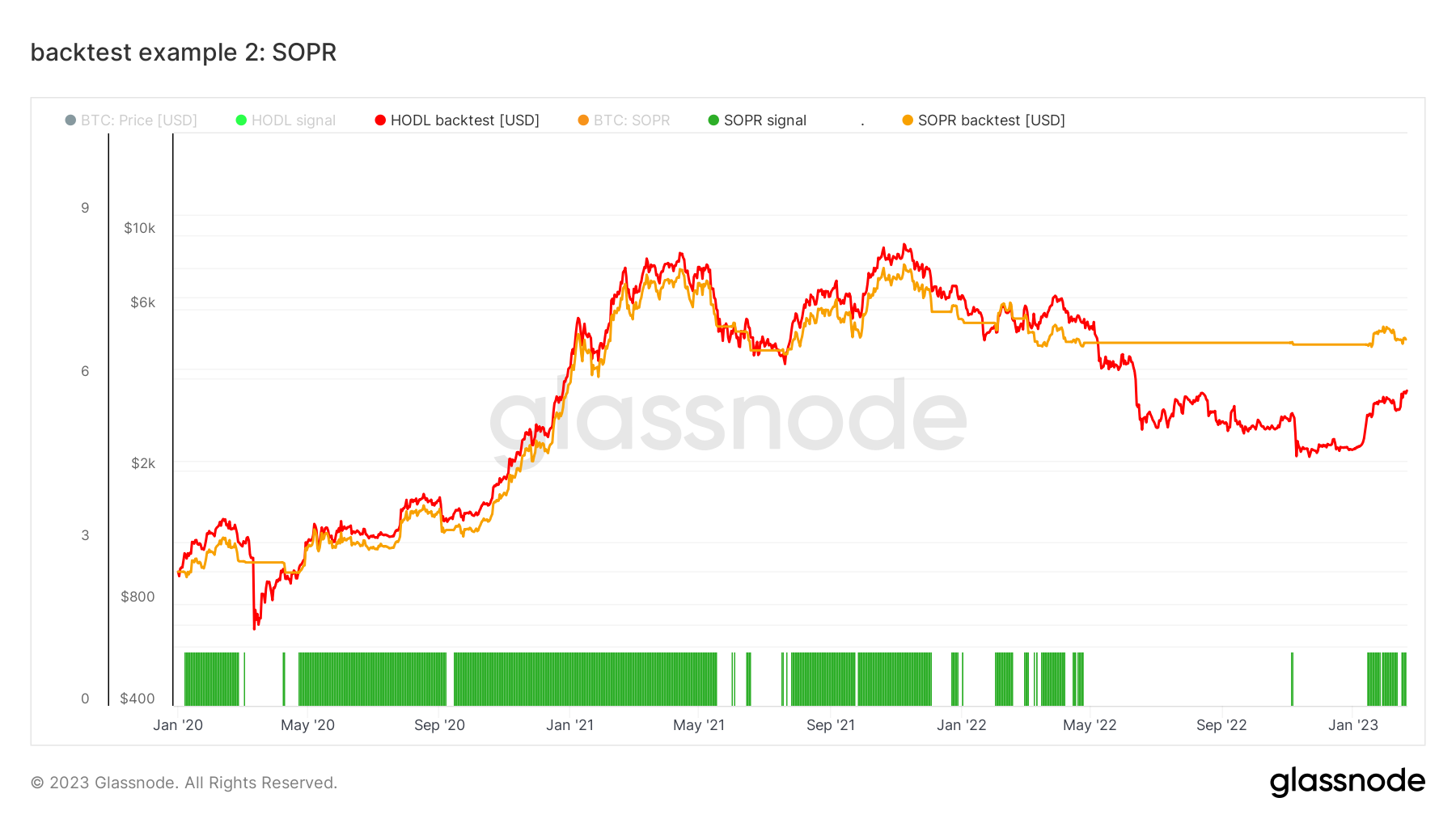
Example 2: an on-chain trading hypothesis based on SOPR
The simple moving average cross-over uses price as the sole input metric. Given only this basic information, it does a reasonable job of identifying trends. However, Bitcoin's public ledger offers way deeper insights into the investors’ behavior than the price alone. The Spent Output Profit Ratio (SOPR), for example, is computed by dividing the realized value (in USD) divided by the value at creation (USD) of a spent output. Or simply: price sold / price paid. Its value informs us whether the average investor sells at a profit (SOPR > 1) or a loss (SOPR < 1). One might deduce that an environment where the average investor sells at a profit is preferable for holding bitcoin compared to when the average investor sells at a loss. Therefore, we define the SOPR-based trading hypothesis (in Python-style pseudo-code for illustration) as:
# SOPR-based trading rules:
if sopr > 1:
    signal = 1
else:
    signal = 0
Let’s look at a backtest. We have prepared a Workbench preset for you with all the ingredients. The SOPR signal is quite noisy; thus, we smooth it with an exponential moving average (EMA). It is loaded as m2 in the preset. In analogy to the previous example, we are adopting the if condition to formalize the SOPR trading rules in Workbench syntax:
if(m2, ">", 1, 1, 0)
This is our trading signal f3. We want to be long bitcoin (signal one) when SOPR (m2) is larger than one and otherwise zero. To run the backtest with the just defined SOPR trading signal, we have defined formula f5 in an exact analogy to the previous examples:
backtest(m1, f3, "2020-01-01", 1000, 0.001)
This will directly generate the NAV curve of the backtest, labeled as SOPR backtest [USD] in the chart below.
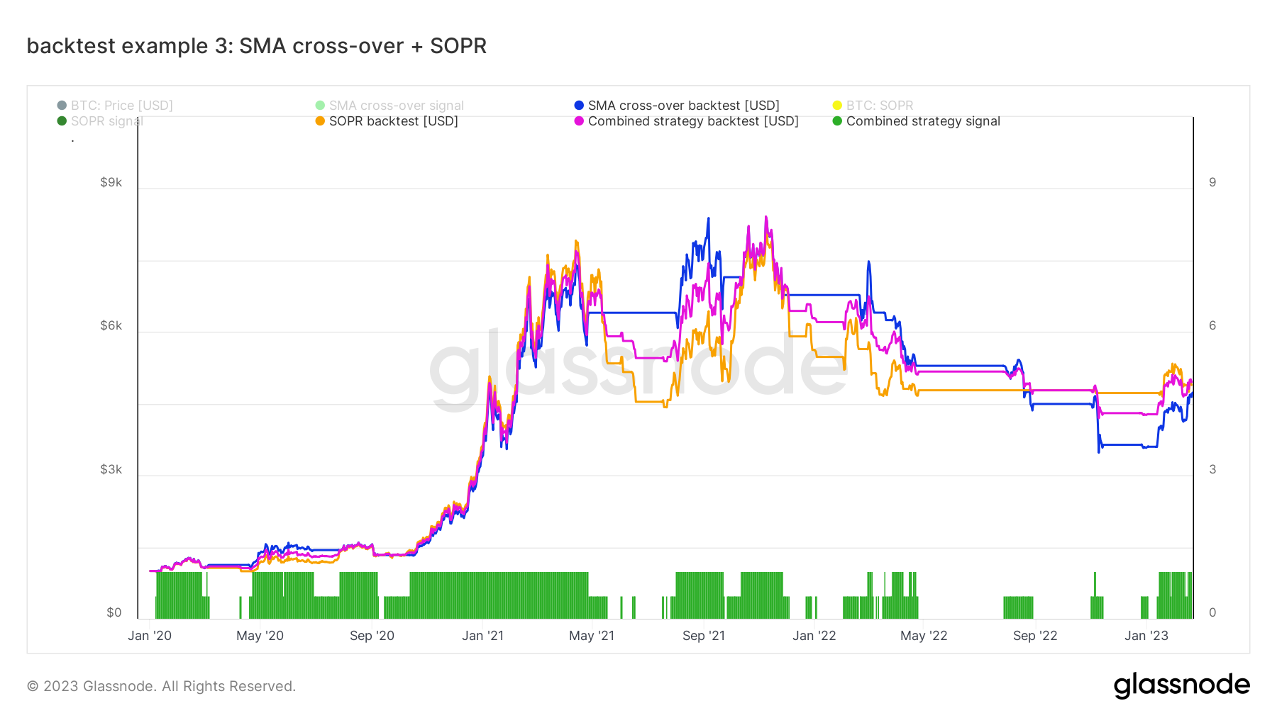
Example 3: combining different trading strategies
We have now explored two trading strategies beyond pure hodling: the SMA cross-over and a strategy based on the SOPR on-chain metric. As the last example of creating a backtest, we look at how one can combine different trading strategy components into one overarching strategy. With multiple strategies, one could imagine splitting the portfolio into several fractions and trading those with different strategies independently. Alternatively, one can combine the strategies based on the individual trading signals beforehand and then trade the combined trading signal for the whole portfolio. In this way, one can save trades when the different components contradict each other. There are no limitations on how to combine different trading signals. The most straightforward way, though, is to average them. Let’s try this out. In the Example 3 Workbench preset, we have defined the SMA cross-over signal as f2 and the SOPR trading signal as f3; then, we can run a combined backtest with:
backtest(m1, (f2+f3)/2, "2020-01-01", 1000, 0.001)
Note how we average the two individual trading signals as input to this backtest.
In the following, we plot the two individual backtests of SMA cross-over and SOPR, labeled as SMA cross-over backtest [USD] and SOPR backtest [USD], respectively, together with the combined backtest. Note how the signal bars Combined strategy signal now not only takes values 0 and 1 but 0.5 in cases where the two strategy components’ signals do not coincide.
What’s next?
This covers the basics of the new backtesting functionality in Workbench. You can make yourself familiar and try out your ideas. You may include short signals in your strategy if you're an advanced trader.
Backtesting doesn’t end with creating a NAV curve. The NAV offers an overview of how an investment would have performed over time. But it does not take the risk of a strategy into account, and neither can one directly read off the relative performance over different periods. Therefore, we introduce the following companion set of functions, which will allow you to get a deeper understanding of your backtest’s performance and allow you to compare different backtests quantitatively:
drawdown(m1)This function takes a backtest result, or any time series, as input and returns the relative drawdown from the all-time high for each point in time. This is analog to the Bitcoin: Price Drawdown from ATH metric.mean_return(m1, period)The annualized rolling mean return of a time series over a given period (in days).realized_vol(m1, period)The annualized rolling realized volatility of a time series over a given period (in days). See also Annualized Realized Volatility.sharpe_ratio(m1, period)The annualized rolling Sharpe ratio is the ratio of annualized rolling mean return and annualized rolling realized volatility. It is one of the most widely used methods for measuring risk-adjusted relative returns.
Note that all functions of the backtesting suite are described in the Workbench Guide, too. In this Workbench preset, we showcase the drawdown and realized_vol functions. We compare the depth of the drawdowns from the HODL strategy (example 0) to the SOPR strategy (example 2). Moreover, we compare the annualized realized volatility of the two strategies. We find that the SOPR strategy has significantly reduced drawdowns compared to a plain HODL investment, and the realized volatility is also highly reduced on a one-year rolling basis.
Disclaimer: The Content of this article and the introduced backtesting functions are for informational purposes only, you should not construe any such information or other material as legal, tax, investment, financial, or other advice. Past performance is fictional, for illustrative purposes only and no indication of future performance.
The introduced functions and features are in a free beta version state and are subject for change.
- Join our Telegram channel
- Follow us and reach out on Twitter
- Visit Glassnode Forum for long-form discussions and analysis.
- For on-chain metrics, dashboards, and alerts, visit Glassnode Studio
- For automated alerts on core on-chain metrics and activity on exchanges, visit our Glassnode Alerts Twitter
